Image Processing 9. Blur
3 min read June 24, 2025 #image processing #javascriptImage Processing 1. Introduction
Image Processing 2. Simple transformation
Image Processing 3. Negate filter, channel extraction and inversion
Image Processing 4. Desaturation
Image Processing 5. Color Models
Image Processing 6. Brightness, saturation, contrast, gamma correction
Image Processing 7. Histogram
Image Processing 8. Image scaling
Image Processing 9. Blur
Image Processing 10. Convolution Kernel
Image Processing 10. Convolution Kernel
Let's return to pixel processing and this time explore image blurring algorithms.
![]()
Standard Blur#
Last time, when discussing bilinear image scaling, we sampled 4 pixels in the original image for each new pixel. We blend components with specific coefficients for smooth results. For the Lanczos filter, number of pixels increased to 9, 25, etc.
Blurring works the same way: sample multiple pixels around the current target pixel, then calculate the arithmetic mean for each color component.
for ; y < height; y++
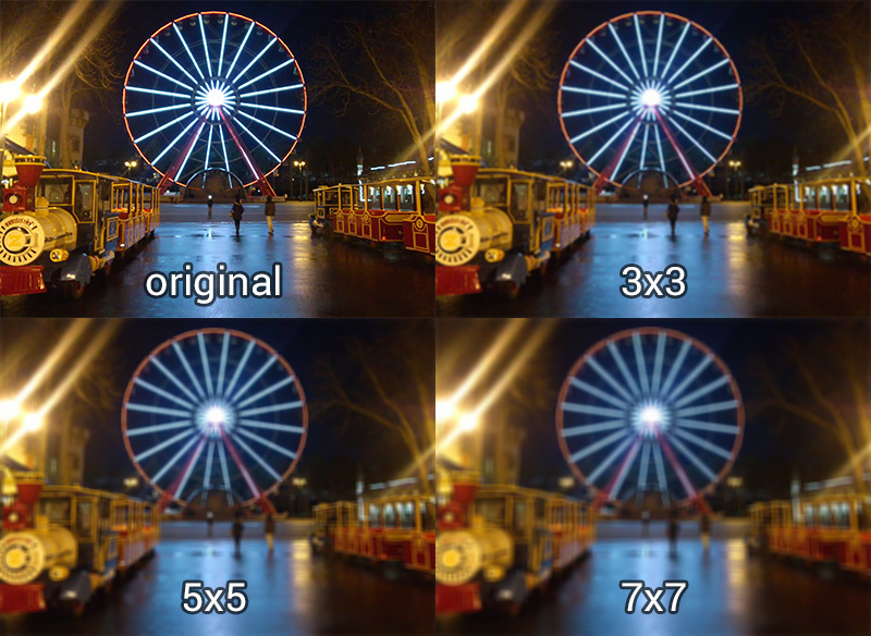
Let's consider a brief calculation. Given a 400×292 image.
- With a normal traversal, we read the pixel 400*292 = 116,800 times.
- With a blur radius of 1 (3×3), we perform 400*292*9 = 1,051,200 reads.
- With a radius of 2 (5×5) – 400*292*25 = 2,920,000 reads
- With a radius of 3 (7×7) – 400*292*49 = 5,723,200 reads
That's a lot! And this isn't even Gaussian blur, which might use 25×25 pixels!
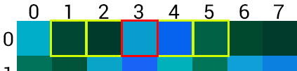
Note on Gaussian Blur
Unlike the method above, Gaussian blur applies decreasing coefficients based on distance from the center. Feel free to modify the code above to account for coefficients. For example, for a radius of 1:
0.2 0.6 0.2
0.6  1  0.6
0.2 0.6 0.2
Box Blur#
There're algorithms that approximate Gaussian blur results. They produce slightly lower quality, but operate significantly faster. For example, you can first blur only in the horizontal direction, then blur the resulting image vertically.

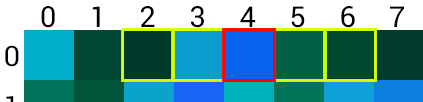
You can also reduce the number of repeated pixel reads. For example, we perform horizontal blurring and are currently at point (0,3). The viewing radius is two pixels (2 left + 2 right + center):
After calculating the sum and dividing by 5, we stored the result at (0,3). Now, move on to processing (0,4):
Last time we already read (0,2), (0,3), (0,4), and (0,5). And these values are already in the sum, so instead of rereading, we subtract the leftmost pixel (0,1) from the sum and add the new right pixel (0,6):
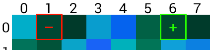
The number of reads is reduced to 2 per pixel (plus 2r+1 for the first pixel in the row). You can go further and replace division by reading a precomputed average value.
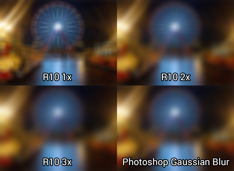
A single pass gives average result, so this filter is typically applied two or more times. Below a comparison between our box blur implementation with a radius of 10 and Photoshop's Gaussian blur with the same radius:
Again, the math. For our 400×292 image the first pass of the optimized algorithm at radius 1 gives 469,276 reads. At radius 2: 470,660, 3: 472,044, 5: 474,812, 10: 481,732, 20: 495,572 reads.
At radius 3, we achieve 12x fewer reads than the unoptimized approach. Even if you perform blurring two or three times, it will still be faster.